Data management and descriptive methods
CASE STUDY: In a clinical trial 12 patients are randomly assigned to two different treatments. Blood measurements are taken before and after the treatment. Load the study1.csv data frame into the R workspace.
study1<-read.table("./data/study1.csv",sep=";",header = TRUE) # the values are separated by ; in the csv fileExercises
Execrise 1.1
Calculate mean, median, variance, standard deviation, quartiles and the sum of the measurements before treatment (mean()).
X<-study1$before
# we will show the direct function and the calculation behind it
# sum of the elements of the vector
sum(X)
## [1] 5.212638
# the sample mean
sum(X)/length(X)
## [1] 0.4343865
mean(X)
## [1] 0.4343865
# the sample variance
sum((X-mean(X))^2)/(length(X)-1)
## [1] 0.01246266
var(X)
## [1] 0.01246266

# the sample standard deviation
sqrt(var(X))
## [1] 0.1116363
sd(X)
## [1] 0.1116363

#the median
mean(sort(X)[c(length(X)/2,length(X)/2+1)])
## [1] 0.4119027
median(X)
## [1] 0.4119027

# quantile
quantile(X, probs=c(0.25, 0.50, 0.75))
##       25%       50%       75%
## 0.3638939 0.4119027 0.5452815
# A quartile is the value of the quantile at the probabilities 0.25, 0.5 and 0.75.

# all of this can be achieved easily using the summary function
summary(X)
##    Min. 1st Qu.  Median    Mean 3rd Qu.    Max.
##  0.2715  0.3639  0.4119  0.4344  0.5453  0.5828
Exercise 1.2
Plot a boxplot and a histogram of the measurements obtained before the treatment. Correct the title of the axes. Choose appropriate range of axes (boxplot()).
par(mfrow=c(1,2))# define the plot area one row, two columns
X<-study1$before
boxplot(X,
        xlab = "Before treatment",
        ylab = "Blood measurements",
        ylim = c(0.2, 0.7),
        main = "Box plot",
        horizontal = TRUE)
points(X, y = rep(0.6, 12), pch=1,
       col="orange", cex=0.75)
# Histogram
hist(X,
     xlim = c(0.2, 0.7),
     xlab = "Before treatment",
     main = "Histogram",
     breaks = 12)
points(X, rep(0, 12), pch=15, col="orange", cex=0.75)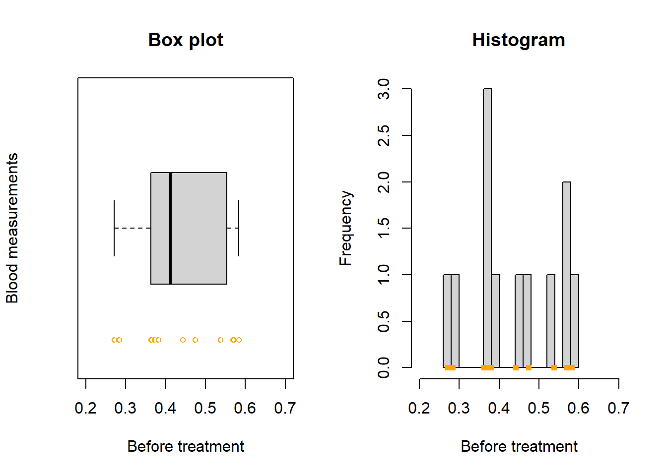
Exercise 1.3
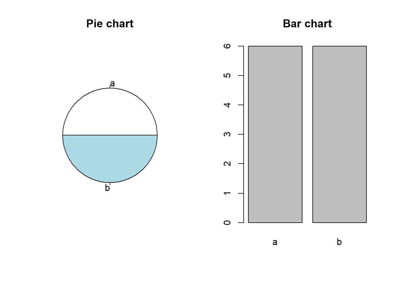
Determine the absolute and relative frequencies of patients in the study groups(table()). Plot a bar chart and a pie chart of the parameter “group” (pie() and barplot()).
X<-study1$group
## absolute and relative
table(X); table(X) / length(X)
## X
## a b
## 6 6
## X
## a b
## 0.5 0.5par(mfrow=c(1,2))# define the plot area one row, two columns
pie(table(X),
main = "Pie chart"
)
barplot(table(X),
main = "Bar chart"
)