Correlation and Regression
Exercise
Exercise 6.1 (Correlation)
Assume Proteins A, B and C are members of a cellular pathway that is related to a certain disease. The concentration of these protein was measured in \(n=5000\) patients.
Read the corresponding data study2.csv into the R-environment.
X = read.table("data/study2.csv", sep=";", header=TRUE)
str(X)
## 'data.frame': 500 obs. of 3 variables:
## $ Protein.A: num 10.7 11.7 10.3 11.9 10 ...
## $ Protein.B: num 13.5 14.8 12.8 14.4 13.2 ...
## $ Protein.C: num 7.06 7.34 8.73 6.53 7.68 ...Make scatter plots of each pair of proteins (plot).
plot(X)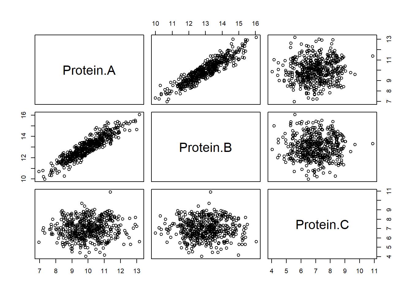
Determine Pearson’s correlation between each pair of proteins (cor.test).
cor.test(X$Protein.A, X$Protein.B)
cor.test(X$Protein.A, X$Protein.C)
cor.test(X$Protein.B, X$Protein.C)
##
## Pearson's product-moment correlation
##
## data: X$Protein.A and X$Protein.B
## t = 50.271, df = 498, p-value < 2.2e-16
## alternative hypothesis: true correlation is not equal to 0
## 95 percent confidence interval:
## 0.8982970 0.9273551
## sample estimates:
## cor
## 0.9139905
##
##
## Pearson's product-moment correlation
##
## data: X$Protein.A and X$Protein.C
## t = 1.9296, df = 498, p-value = 0.05423
## alternative hypothesis: true correlation is not equal to 0
## 95 percent confidence interval:
## -0.00155775 0.17253187
## sample estimates:
## cor
## 0.08614461
##
##
## Pearson's product-moment correlation
##
## data: X$Protein.B and X$Protein.C
## t = 0.28971, df = 498, p-value = 0.7722
## alternative hypothesis: true correlation is not equal to 0
## 95 percent confidence interval:
## -0.0747947 0.1005572
## sample estimates:
## cor
## 0.01298103Exercise 6.2 (Linear Regression)
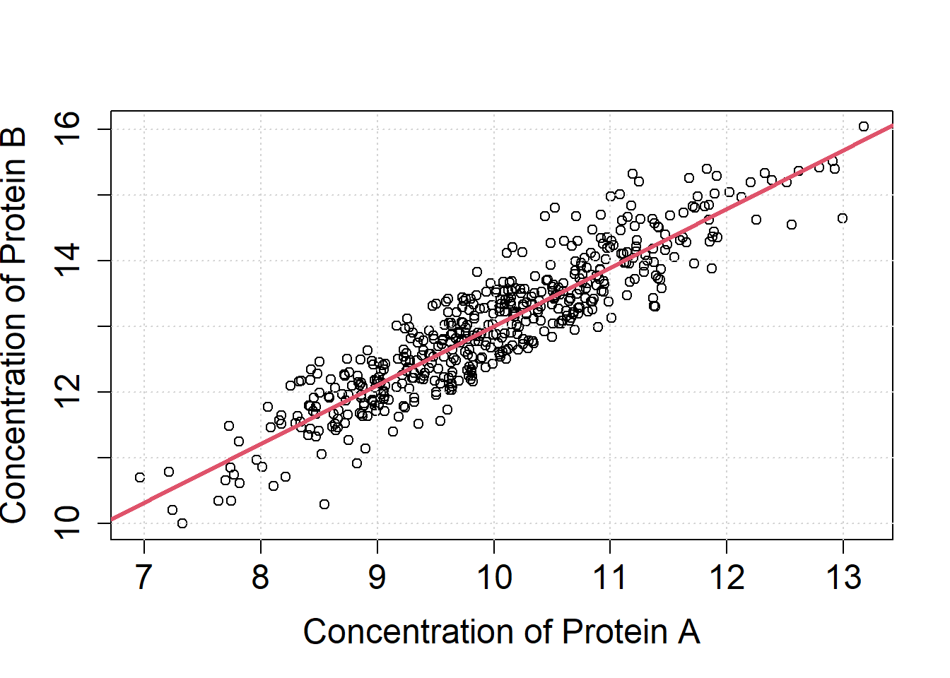
From the correlation analysis, protein A appears to be related to protein B. From earlier research, it is known that protein B depends on protein A. Model the relation between the two proteins using a simple linear regression (lm).L1 = lm(X$Protein.B ~ X$Protein.A)Evaluate the summary over the linear model to check the goodness of fit.
summary(L1)##
## Call:
## lm(formula = X$Protein.B ~ X$Protein.A)
##
## Residuals:
## Min 1Q Median 3Q Max
## -1.41408 -0.30749 0.00183 0.28727 1.33353
##
## Coefficients:
## Estimate Std. Error t value Pr(>|t|)
## (Intercept) 4.03927 0.17893 22.57 <2e-16 ***
## X$Protein.A 0.89633 0.01783 50.27 <2e-16 ***
## ---
## Signif. codes: 0 '***' 0.001 '**' 0.01 '*' 0.05 '.' 0.1 ' ' 1
##
## Residual standard error: 0.4258 on 498 degrees of freedom
## Multiple R-squared: 0.8354, Adjusted R-squared: 0.835
## F-statistic: 2527 on 1 and 498 DF, p-value: < 2.2e-16Do you know the meaning behind each section of summary?
T-statistic
The t-Test checks the nullity of the coefficient.
Multiple R-squared
Percentage of variability explained by the model.
F-statistic
The F-Statistic checks if at least one of the coefficients is nonzero, namely the null hypothesis is that all of the regression coefficients are equal to zero.
The output of the lm is a list which contains the estimates of the linear regression model. Use the latter to draw the regression line into the scatter plot (abline).
par(mfrow=c(1,1))
plot(X$Protein.A, X$Protein.B, cex.axis=1.5, cex.lab=1.5,
     xlab="Concentration of Protein A",
     ylab="Concentration of Protein B")
grid()
#The coefficients of the linear regression model
#L1$coefficients
abline(a=L1$coefficients[1], b=L1$coefficients[2], col=2, lwd=3)