Analysis of variance
Theory
Let’s consider the framework in which there are k levels of a factor of interest, which identify k different groups of observations.
The statistical model for one-way analysis of variance is: \[ y_{ij}=\mu+\tau_{i}+\epsilon_{ij}\quad i=1,\dots,k \text{ and } j=1,\dots,n_{i} \] where \(\mu\) is the general mean, \(\tau_{i}\) is the treatment effect for group \(i\) and \(\epsilon_{ij}\sim N(0,\sigma^2)\). By considering a suitable F-test is possible to test the null hypothesis that all mean are equal (\(\tau_i=0\;\forall i\)) against at least one treatment effect not null. To perform this test we use the aov function.
Formulas in R
The the formulas in R are used to specify the symbolic model as well as generating the intended design matrix. The formula are characterized by the \(\sim\) as you can see in this example y~x.
Let y and x1 be two variables, with y~x1we mean that y, the dependent variable, depends on x1, the independent variable. When the dependence relation is quadratic will write y~I(x1^2), indeed you nedd to use I(), as-is operator, to apply a function to a variable. Now let x2 be another variable, withy~x1+x2we mean that y depends on x1 and x2 but there is no dependence between x1 and x2. We will use the \(-\) sign to ignore an object in the analysis, e.g. y~x1-1 delete the intercept (regress through the origin). If we want to express the dependence of y on x1, x2 and their interaction we will write y~x1+x2+x1:x2, the former is equal toy~x1*x2.
Exercises
Exercise 8.1 (One-way analysis of variance)
Assume the concentration of a certain metabolite was measured in three experimental groups.
Sample sizes:
n1 = 12
n2 = 18
n3 = 8
Mean concentration in the population from which samples were drawn:
mu1 = 1
mu2 = 4.5
mu3 = 6
Measurement values can be generated using normal distribution:
x1 = rnorm(n=n1, mean=mu1, sd=3)
x2 = rnorm(n=n2, mean=mu2, sd=3)
x3 = rnorm(n=n3, mean=mu3, sd=3)- Plot the concentration versus the group levels (boxplot).
boxplot(x1, x2, x3, cex.lab=1.5, cex.axis=1.5, xlab="Group",
        ylab="Concentration (mg/ml)", names=c(1, 2, 3), lwd=2)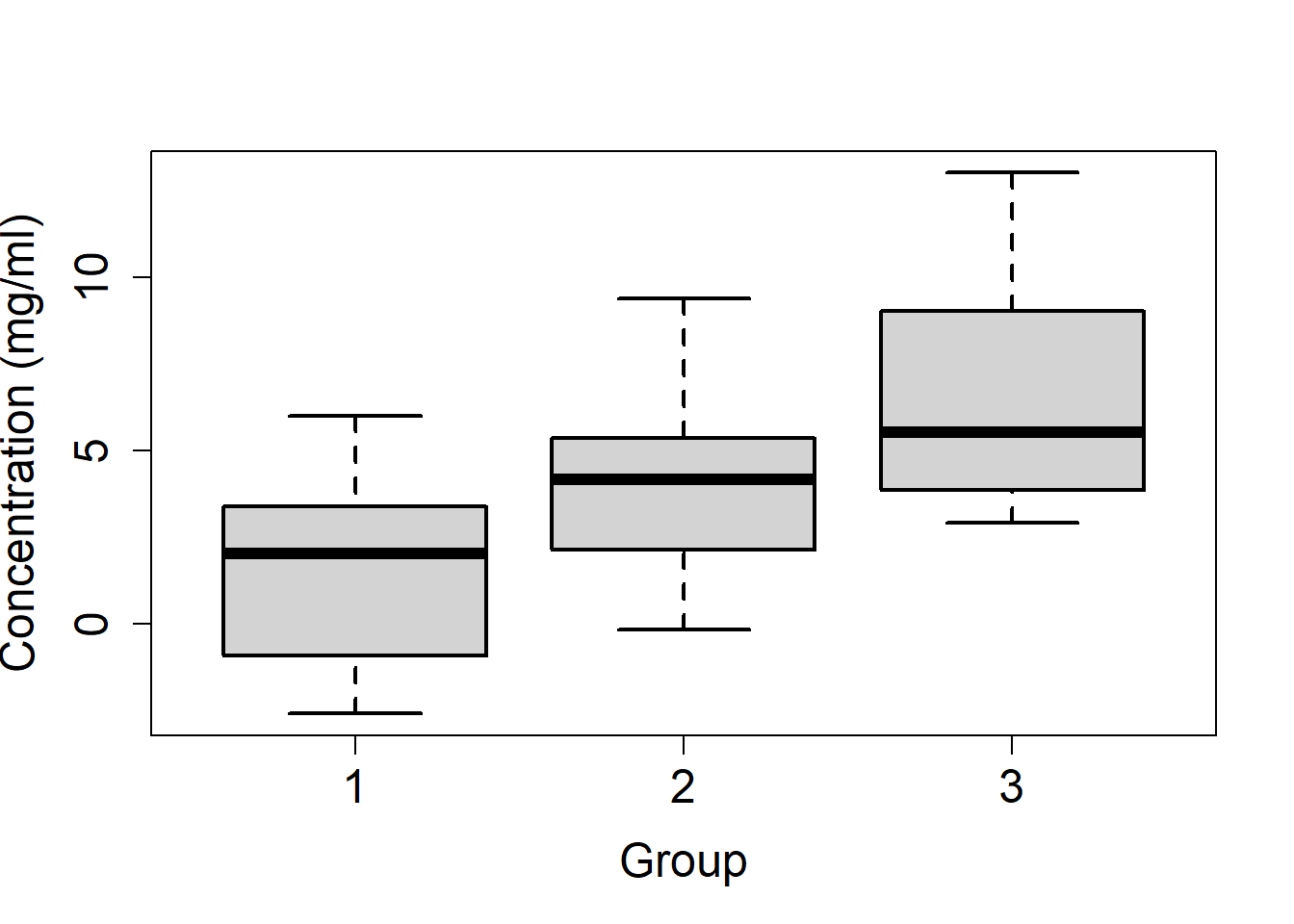
- Perform one-way analysis of variance (aov).
x = c(x1, x2, x3)
group = (c(rep('1', n1), rep('2', n2), rep('3', n3)))

aov.oneway = aov(x ~ group)
summary(aov.oneway)
## Df Sum Sq Mean Sq F value Pr(>F)
## group 2 125.1 62.53 7.637 0.00177 **
## Residuals 35 286.6 8.19
## ---
## Signif. codes: 0 '***' 0.001 '**' 0.01 '*' 0.05 '.' 0.1 ' ' 1What dose the result suggest?
(EXTRA) Plot the stripplot of the the data set to add the mean values of each group and to draw the segments connecting them. To do this, use the coefficients of the output given by the function summary applied to the object obtained from aov .
plot(x ~ group,
     xlab="Group",
     ylab="Concentration (mg/ml)",
     pch=16)

# mean of the first group
tr1<-summary.lm(aov.oneway)$coefficients[1,1]
# mean of the second group
tr2<-tr1+summary.lm(aov.oneway)$coefficients[2,1]
# mean of the second group
tr3<-tr1+summary.lm(aov.oneway)$coefficients[3,1]

points(c(1,2,3),c(tr1,tr2,tr3),col='red',lwd=2)
lines(c(1,2,3),c(tr1,tr2,tr3),col='red',lwd=2)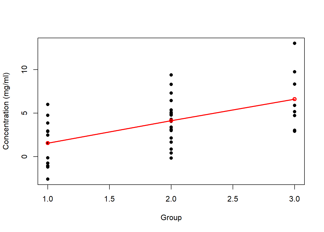
- Perform subsequent pairwise group comparisons by t-tests to see which groups are different. As the chances of committing a type I error for a series of comparisons is greater than the error rate for any one comparison alone, use the Bonferroni correction to lower down the family-wise error rate.
t1 = t.test(x1, x2,conf.level = 1-0.05)
t2 = t.test(x1, x3,conf.level = 1-0.05)
t3 = t.test(x2, x3,conf.level = 1-0.05)

c(t1$p.value, t2$p.value, t3$p.value)<=0.05/3
## [1] FALSE TRUE FALSE- Repeat the exercise with increased variances in the measurement values (e.g. sd = 5).
x1 = rnorm(n=n1, mean=mu1, sd=5)
x2 = rnorm(n=n2, mean=mu2, sd=5)
x3 = rnorm(n=n3, mean=mu3, sd=5)

x = c(x1, x2, x3)
group = (c(rep('1', n1), rep('2', n2), rep('3', n3)))

aov.oneway = aov(x ~ group)
summary(aov.oneway)
## Df Sum Sq Mean Sq F value Pr(>F)
## group 2 13.0 6.482 0.313 0.734
## Residuals 35 725.6 20.731Exercise 8.2 (Repeated measurements analysis of variance)
Some concentration was measured in \(n = 10\) patients repeatedly at \(T = 4\) time points. Load the dataset Repeated_OneWay.csv.
X <- read.csv("./data/Exercise_8_3_Repeated_OneWay.csv", sep=";")
str(X)
## 'data.frame': 40 obs. of 3 variables:
## $ Patient : int 1 2 3 4 5 6 7 8 9 10 ...
## $ Time : int 1 1 1 1 1 1 1 1 1 1 ...
## $ Concentration: num 2.44 2.77 4.56 3.07 3.13 ...- Plot the concentration across different time-points. Use one-way repeated measures ANOVA to detect whether there is a time effect without the information of repeated measures.
boxplot(X$Concentration ~ X$Time,
        xlab="Time",
        ylab="Concentration")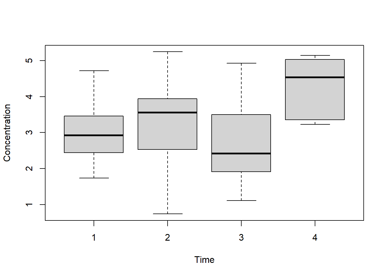
summary(aov(X$Concentration ~ X$Time))## Df Sum Sq Mean Sq F value Pr(>F)
## X$Time 1 4.57 4.569 3.51 0.0687 .
## Residuals 38 49.47 1.302
## ---
## Signif. codes: 0 '***' 0.001 '**' 0.01 '*' 0.05 '.' 0.1 ' ' 1- Perform one-way repeated measures ANOVA with information of repeated measures. This is equal to add a random effect to the model that keeps in mind the correlation between observation from the same patient, random effects model. To do this, wrap the relevant variable inside Error() operator and add it to the formula.
summary(aov(X$Concentration ~ X$Time + Error(X$Patient)))##
## Error: X$Patient
## Df Sum Sq Mean Sq F value Pr(>F)
## Residuals 1 0.5788 0.5788
##
## Error: Within
## Df Sum Sq Mean Sq F value Pr(>F)
## X$Time 1 4.57 4.569 3.458 0.0709 .
## Residuals 37 48.89 1.321
## ---
## Signif. codes: 0 '***' 0.001 '**' 0.01 '*' 0.05 '.' 0.1 ' ' 1- A second group was studied in the above study. Plot the concentration versus the group levels across different time-points. Analyse whether there is an effect by time, group or an interaction between time and group (boxplot). Data is given in the folder Repeated_TwoWay.csv.
X = read.csv("./data/Exercise_8_3_Repeated_TwoWay.csv", sep=";")
str(X)

boxplot(X$Concentration ~ X$Time + X$Group,
        xlab="Time",
        ylab="Concentration",
        col=c(2,2,2,2,3,3,3,3)
        )

#3.1 means time 3 group 1

legend("topleft", c("Group 1", "Group 2"), col=c(2,3), ncol=2, pch=15)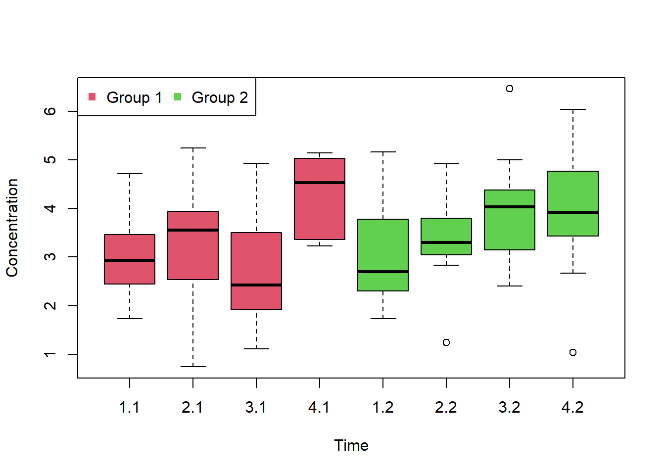
## 'data.frame':    80 obs. of  4 variables:
##  $ Patient      : int  1 2 3 4 5 6 7 8 9 10 ...
##  $ Time         : int  1 1 1 1 1 1 1 1 1 1 ...
##  $ Concentration: num  2.44 2.77 4.56 3.07 3.13 ...
## $ Group : int 1 1 1 1 1 1 1 1 1 1 ...- Conduct Anova without information of repeated measures. Also, conduct Anova with information of repeated measures.
#Without information of repeated measures; and with intreacttions
summary(aov(X$Concentration ~ X$Time + X$Group + X$Time:X$Group))

### With information of repeated measures
summary(aov(X$Concentration ~ X$Time + X$Group + X$Time:X$Group + Error(X$Patient)))
## Df Sum Sq Mean Sq F value Pr(>F)
## X$Time 1 10.60 10.595 7.771 0.0067 **
## X$Group 1 0.83 0.834 0.612 0.4366
## X$Time:X$Group 1 0.05 0.054 0.039 0.8431
## Residuals 76 103.62 1.363
## ---
## Signif. codes: 0 '***' 0.001 '**' 0.01 '*' 0.05 '.' 0.1 ' ' 1
##
## Error: X$Patient
## Df Sum Sq Mean Sq F value Pr(>F)
## Residuals 1 0.4954 0.4954
##
## Error: Within
## Df Sum Sq Mean Sq F value Pr(>F)
## X$Time 1 10.60 10.595 7.705 0.00695 **
## X$Group 1 0.83 0.834 0.607 0.43855
## X$Time:X$Group 1 0.05 0.054 0.039 0.84372
## Residuals 75 103.13 1.375
## ---
## Signif. codes: 0 '***' 0.001 '**' 0.01 '*' 0.05 '.' 0.1 ' ' 1